
By calculating the daily rate of change in the extra-tropics as the length of day changes throughout the year, it is possible to use this data when added to the clear sky daily solar input for that location to generate an actual measured climate sensitivity.
Data source:
ftp://ftp.ncdc.noaa.gov/pub/data/gsod/
Code and reports (chart source data):
http://sourceforge.net/projects/gsod-rpts/
I started with the day to day change in both min (mndiff) and max (mxdiff) temps for each day of the year.

This is the derivative of temperature by day, the maximum peaks in March in the northern hemisphere, the negative peak happening in October, the slope between peaks is calculated with the PL/SQL Slope function between March and October as Cooling, and from October to March as Warming.

This is an over lay of the day to day change in temp for all stations in the US 1950-2010.
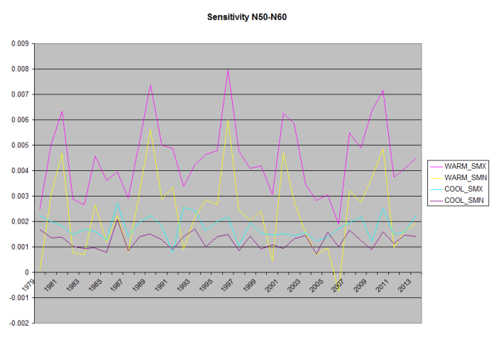
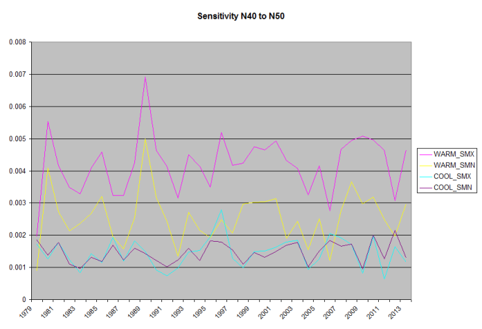
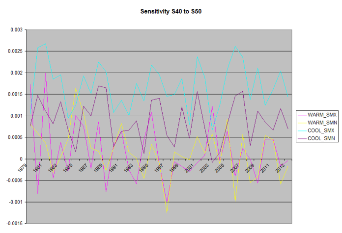
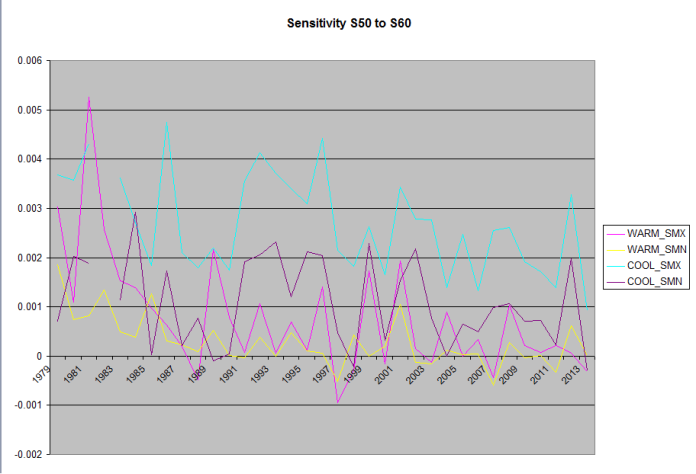
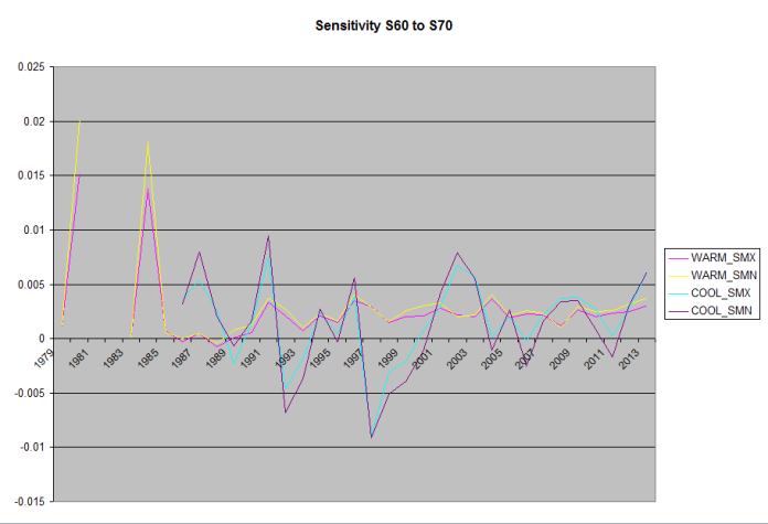
Taking the slope of the change in temperature as the length of day is changing and then dividing that by the slope of daily solar input in Whr/m^2/day (Work/Day/Watt), gives us an actual Climate Sensitivity. This is the response in Temp F°/Whr/m^2/day (divide by 43.2 to get the instantaneous rate in C° ) at that station. A collection of stations based on area are then averaged together.
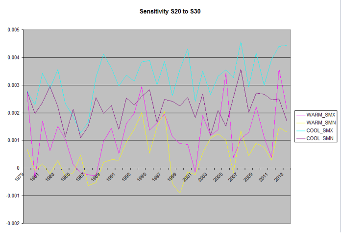
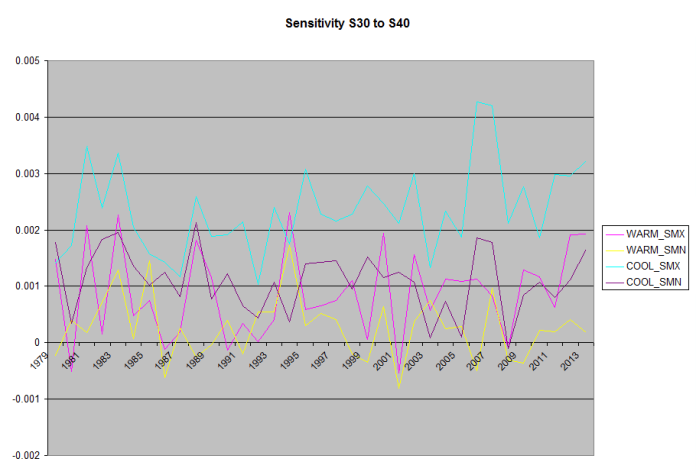
Because the daily Solar input is strongly dependent on Latitude, I’ve calculated and graphed this for 10 degrees latitude bands starting @N/S 20 going to N/S 90, no stations north of N80 meet the inclusion requirements (360 days per year collecting samples by station).

Temp F°/Whr/m^2/day
Temp F°/Whr/m^2/day
Temp F°/Whr/m^2/day

Temp F°/Whr/m^2/day

Temp F°/Whr/m^2/day
Note, because the Southern Hemisphere’s seasons are reversed, the Warming/Cooling labels are backwards.
Temp F°/Whr/m^2/day
Temp F°/Whr/m^2/day
Temp F°/Whr/m^2/day
Temp F°/Whr/m^2/day
Temp F°/Whr/m^2/day

Hi Michael,
I would like to thank you to your great contribution to Facebook today.
Your post on solar radiance effect to global warming was great!
I was wondering if you are thinking of publishing?
Anyway keep up the good work,
Jimmy
LikeLike
Micro: I followed your link here from WUWT. Not every ratio measuring a change in radiation (a potential forcing) and a change in temperature should be interpreted as a “climate sensitivity” especially as an “equilibrium climate sensitivity”. If you understand dimensional analysis or the factor-label method, the physics reasons for this mistake should become apparent:
Forcing is measured in units of power/area or energy/time/area. Temperature is proportional to energy/volume (or energy/weight and density) and the proportionality constant is called heat capacity (K/m^3). To obtain the temperature change produced by a forcing, you need to specify the amount of TIME the forcing is applied (to convert power to energy) and the DEPTH of the material being warmed by the forcing (to convert area to volume).
It is an interesting exercise to calculate the rate at which an radiative imbalance of 1 W/m2 can uniformly warm a planet with a mixed layer of ocean 50 m deep covering 70% of the surface. The mixed layer is the effective depth of ocean that warms every summer. (If you want, include the heat capacity of the atmosphere and estimate it for a thin layer of soil, but the bulk of the heat capacity is in the ocean.) You should get an initial rate of 0.2 K/yr. I say an “initial rate” because – as soon as the surface begins to warm, increased radiative cooling from a warmer planet reduces the radiative imbalance and the rate of warming starts to slow. (The rate of slowing depends on ECS.) And if you consider periods longer than a season, significant amount of heat are transported below the mixed layer.
Nevertheless, many people recklessly convert forcing or radiative imbalance into a temperature change using ECS. WIllis and “Spot the Volcano”, for example.
So how do climate scientists get around this dilemma posed by dimensional analysis? First, they convert power into energy by integrating the area under the radiative imbalance (which shrinks with warming) vs time curve until the imbalance reaches zero – equilibrium! The further into the ocean heat penetrates, the longer it takes to reach equilibrium – but the equilibrium warming doesn’t change. So, the only way one can rigorously convert a forcing into a temperature change (using the laws of physics) is when warming has reached equilibrium. Needless to say, that takes a long time. It doesn’t happen in one season or one decade.
To avoid this slow approach to equilibrium, climate scientists invented a different measure of climate sensitivity, transient climate response. At the end of a long period of rising forcing, the deep ocean will not have come into equilibrium with the warmer surface. At equilibrium, the earth has warmed enough so that the entire forcing (dF) has been negated by more OLR leaving for space (and more SWR being reflected to space). Before equilibrium, some of the radiative imbalance is going into warming the ocean (dQ) and the warming is sending the rest to space.
dW = lambda*dT
dF/dT_eq = (dF-dQ)/dT_transient
ECS = dT_eq/dF
TCR = dT_transient/(dF-dQ)
If you look at your second Figure, land surface temperature peaks about 1 month after peak irradiation. This is because the heat capacity over land (especially away from the coast) than it is over the ocean. If you look at SST, there will be a much bigger lag. In the Arctic, were melting sea ice creates the biggest heat capacity, minimum sea ice occurs in September, almost 90 degrees out of phase with radiation. In all cases, you need to remember that the heat delivered by SWR does not stay at the latitude of location it is received, it is transported both longitudinally (trade winds, jet stream) and latitudinally.
LikeLiked by 1 person
I’ll have to look at this again. But did you look at the measured change in radiation in the nonlinear cooling link?
LikeLike
The second figure is dT/day, and the cross over isn’t delayed other than by weather. It is hard to see but, dT/day approximately crosses zero right around the end of June, as the days start to shorten. The slope of that line is dT, and the for effective sensitivity, I divide that by the slope of the change is solar forcing for clear skies. My data set does not have surface solar, so i used pmod solar data to calculate w/m^2. So you see the response of temperature.
LikeLike
While station solar forcing is a calculation, it’s based on measured TSI (pmod), and the temp change is measured change. Now, maybe enthalpy would be better than temps, and I can do that, but I found enthalpy really just follows temperatures, mostly as one would expect.
LikeLike
The math here is hogwash . You have to integrate the the fluxes over entire surface area to get a complete flux and then use the Stefan Boltzmaan equation to get a temperature because of the 4th power problem . this is the only way to circumvent the Holder inequality problem see the Den Volokin paper on this . It is Ned Nikolov’s name spelled backwards. Unless you get around Holder’s inequality your math is bullshit.
LikeLike
While I hadn’t applied the process here, I did start coding to do all of my temp math by 1st converting it into a flux, doing my equations, and then converting it back to a temp. So good point. But since day to day change is small, the error should also be fairly small (fingers crossed, hogwash feels a touch harsh 🙂 ).
I figured out that the daily cooling process regulates temps with wv, co2 has no little to affect. And I got busy at work and stopped working on my time series code a couple years ago.
But I do appreciate you pointing this out, few even acknowledge it.
I will also note that the wv cooling regulation work shoots a large hole in GHG theory, and doesn’t invalidate Ned’s work. I don’t have the knowledge to tell if Ned is “right” or not. But this might move me further his way. It’s here https://micro6500blog.wordpress.com/2016/12/01/observational-evidence-for-a-nonlinear-night-time-cooling-mechanism/ if you hadn’t looked at it.
LikeLike